As explained by Jon in his previous post, we are using precomputed global illumination in The Witness, and one of my first tasks was to work on that system.
I have developed some interesting technology to compute automatic paramaterizations, to formulate the lighting computations in a way that can be easily mapped to the GPU, and to speed them up performing them at a lower frequency by using irradiance caching. None of these things are very cutting edge, but I run into some interesting problems that are usually overlooked in the literature and came up with some creative solutions that I think would be interesting to share. However, in retrospect, I think I also made some mistakes, but I hope that being honest about them will help me avoid them in the future.
In this first post I will describe the lightmap parameterization algorithm that I have implemented and in the next few posts I’ll cover other details of our lighting system such as our approach to perform final gathering using hemicubes and our implementation of irradiance caching.
In order to use precomputed lighting we need a way of mapping these lighting computations to the surfaces. One possibility is to store them per vertex, but in many cases that does not provide enough resolution and the interpolation of the lighting makes the triangulation of the mesh fairly obvious. Many games get away with that by compensating the lack of detail in the lighting with high texture and normal map detail, but that does not go along well with the graphical style that Jon wants to achieve. So, instead of that we decided to create full parameterizations of our objects in order to store the precomputed lighting into lightmap textures.
Creating these parameterizations by hand is possible, but it is time consuming and I’d rather have our artists work on something more enjoyable. So, we decided to create the parameterizations automatically. However, the greatest mistake I’ve made so far is to not look more carefully at the available solutions to accomplish that. I had some pieces of the implementation already available, and I overestimated how much effort it would take to put them together and produce robust results. While talking about this to some friends at GDC one of them asked why I wasn’t using Microsoft’s UVAtlas tool, and to my dismay and embarrassment my only answer was that it had not occurred to me. I think that goes to prove how valuable it is to be open about our development in a small team like ours.
Now that I got that out of the way, let’s talk about the tech. We only use lightmaps to represent indirect illumination and the direct illumination of static area lights. So, our expectation was that lightmaps would be fairly smooth and that seams would not be a huge problem. For this reason we decided not to invest in a solution that guaranteed seamless parameterizations and instead used a fairly traditional approach: We first divide the input geometry into charts with disk topology, parameterize them individually, and finally pack them into a rectangular texture.
Segmentation
Dividing the mesh into charts is by far the most complex step of the process. In the past I had tried using hierarchical clustering without much success, so this time around I decided to use an iterative clustering algorithm similar to Lloyd’s algorithm, in the same vein as the algorithm used in the Multi-chart geometry images (MCGI) paper.
Like Lloyd’s clustering algorithm, the MCGI algorithm iterates between chart growing and reseeding stages. The growth of the charts is guided by a metric based on the normal deviation and the distance between the face centroids. After each chart growing iteration a new seed is selected taking the most central face of the chart, and the process is repeated until the seed location does not change anymore.
My implementation of the MCGI algorithm worked moderately well, but it didn’t always produce good results. It was possible to tweak the number and location of the seeds to obtain the desired output, but that required a certain amount of user intervention that was not desired.
Part of the problem is that the meaning of “good” in this setting is very subjective. It usually means nicely shaped charts, that fit well to the surface, produce parameterizations with little distortion, have fairly straight and convex boundaries and are more or less equaly sized.
In order to adapt the algorithm to our purposes I did two things, modified the bootstraping method so that the initial number of seeds is chosen automatically and used a combination of metrics to obtain better control over the results.
In order to select the initial number of seeds, I simply insert the seeds one by one, and grow the respective charts until a threshold is met. At that point I pick an arbitrary face that is not assigned to any chart yet and repeat the process. When no faces are left, the growing process is restarted from all seeds in parallel.
A common strategy to remove the sensitivity to the initial conditions is to use the farthest point heuristic. However, instead of doing that I found that an approach that works well is to pick the worst candidate face of the already chosen charts as the next seed.
The second important change to the algorithm was to use a different set of metrics. The MCGI paper proposes a metric that combines normal deviation with distance between face centroids. I found that using absolute distances made the algorithm very dependent on the tessellation of the mesh and that measuring the distances from the centroids favored triangles with low aspect ratios.
Instead of using distance between faces I considered only the normal deviation and combined it with other metrics similar to the ones proposed in D-Charts: Quasi-Developable Mesh Segmentation and that take roundness and straightness into account.
These metrics also had their own problems and I had to tweak them in various ways. The most significant issue is that they constrained the chart growth in undesired ways. For example, to encourage chart convexity you would associate a high factor to the corresponding metric, but that would result in a large number of almost convex charts, as soon as a convex configuration was found no additional faces could be added to the chart. So, instead of using these metrics to constrain the growth I only use them to favor convex charts or straight boundaries; that allowed the charts to grow freely, but still retain the most convex and most straight shape possible.
A trick that helped in many cases was to incorporate some input from the artist, but without imposing any additional burden to them. A simple way of doing that is taking into account the existing parameterization of the mesh. Our objects already have a parameterization that is used for texturing and the artists tend to place texture seams at locations that are not easily visible. Snapping the boundaries of our charts to the existing seams did not only reduce the overall number of seams, but also caused the charts to evolve in a way that matches better what the artist would have done manually.
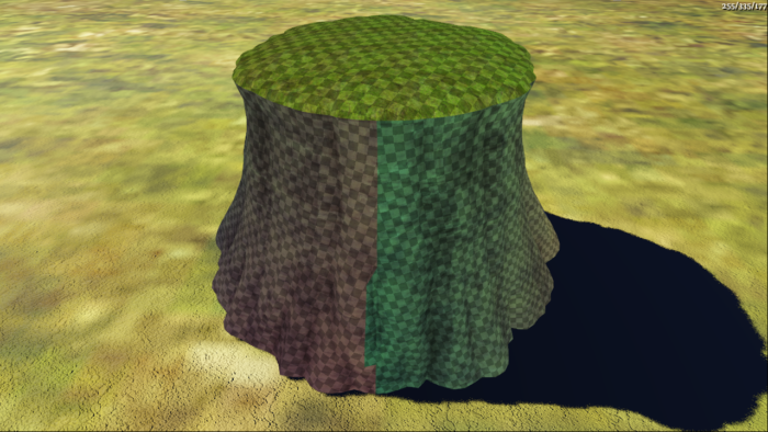
I considered texture and normal seams independently. Since our parameterization is used for lighting I follow normal seams more strictly and proportionally to their angle, not doing so would cause the corners to appear less defined or more blurry. That also helps the process to converge much more quickly in architectural meshes that have many hard edges.
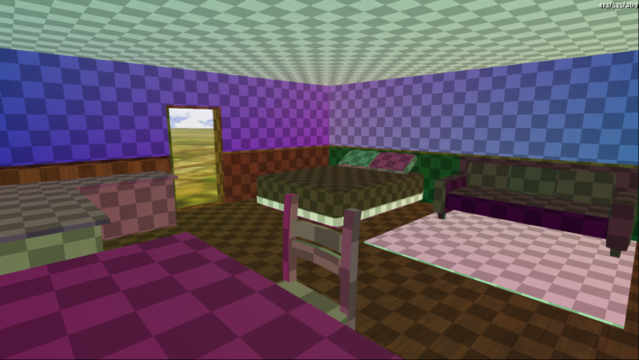
Finally, I don’t impose any chart topology constrains. I specially wanted charts go grow around holes in the mesh as long as the metric was below the desired threshold. I was tempted to use a better proxy fitting metric instead of the normal deviation metric, but that would have generated cylindrical or conical charts that would have to be cut, and I did not want to deal with that. Closing holes on the other side is fairly easy, it’s just matter of detecting the boundaries and closing all, but the longest one.
Parameterization
For the chart parameterization algorithm we simply use Least Squares Conformal Maps since I had an implementation already available. My implementation is based on the description of the algorithm in the notes of the SIGGRAPH 2007 Mesh Parameterization course, which I found much more accessible than the one in the original paper. Particularly useful is the chapter about numerical optimization, although if I had to write a sparse matrix solver again I would probably use OpenNL, since it has now been released under a liberal BSD license.
LSCM is not the best parameterization algorithm out there. It worked pretty well in most cases, although in some rare situations it resulted in small self-overlaps. That happened in two cases:
The first case turned out that was caused by T-junctions in the input mesh that were detected as holes and filled with a degenerate triangle. In practice the small overlaps in the parameterization were not really an issue so instead of fixing the input we simply plan to report these problems to the artist in the exporter and have him fix the them if it turns out it’s causing artifacts.
In the second case, increasing the weight of the convexity metric used during the clustering process allowed us to prevent these errors. So, I didn’t really do anything to handle this problem, but so far it has not been an issue.
Even after that we had some problematic cases remaining. I noticed that the implementation in Blender was not having this same issues and was handling these cases more gracefully. So, I asked Brecht Van Lommel, who suggested the use of alternate matrix weights based on the ABF formulation of LSCM, and that seemed to eliminate the remaining issues.
While LSCM is very easy to implement, it’s definitely not the best parameterization method out there. If I were to implement something better I would probably look at LinABF or Fitting to Guidance Gradient Fields. However, since parameterization of the individual charts is currently the fastest step it may make sense to also look at more expensive deformation analysis methods.
Packing
Our packing algorithm is fairly simple. Like many other implementations we first sort the charts by parametric area, rotate them to align the charts with their best fit rectangle and greedily introduce them in the atlas one by one. Ideally I should test all 4 possible orientations, but currently I simply pick one of the orientations randomly.
Instead of using a tetris-like scheme to find the best location for each chart, I use a more brute force approach in which all the possible locations are considered. I achieve that using a conservative rasterizer that tags all the texels touched by a chart, plus an extra texel for padding. I progressively increase the texture extents as new charts are inserted. If the a location within the current extents is found, the chart is automatically accepted, otherwise a metric is evaluated to determine the location that least increases the extents of the atlas. Since I use a greedy algorithm, minimizing area resulted in atlases with very high aspect ratios. So, instead I minimize a metric that combines extent and perimeter and results in mostly square atlases.
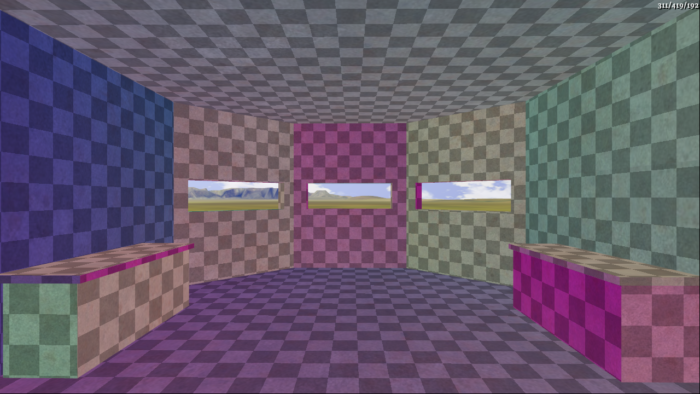
Here are some examples of the results:
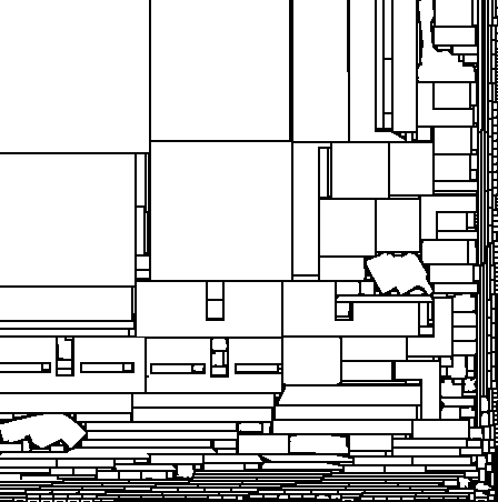
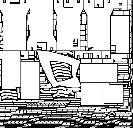
Once we use lightmap compression it will probably make sense to align the charts to DXT block boundaries in order to prevent bleeding artifacts.
Future Improvements
This is one of the areas where I think there’s a lot of room for improvement, but at the same time, there’s not much !/$ in spending more time improving the results. Even though it has not been tested in production, I think that our current solution works fairly well. It would be nice to have larger charts with less distortion or a lower number of seams, and I would certainly have fun working on that. However, that’s not going to make the game run significantly faster or look dramatically better. We plan to release the source code of these algorithms at some point so my hope is that the implementation will progressively get better as other people adopt it and improve it to fit their needs.
That said, if there’s one area where I think it’s worth investing, that is in the use of signal specialized parameterizations. The research papers on the subject (Signal-specialized parametrization and Signal-specialized parameterization for piecewise linear reconstruction) are probably overkill in our setting, and I’m not sure they would work very well with our low resolution meshes.
Half-Life 2 achieved that that by using artist specified sampling rates for each surface, but I think it’s worth doing that automatically using an approach like the one proposed by Bungie, which seems fairly simple and provides most of the gains the more complex approaches would give us.
My expectation is that the current implementation won’t suffer significant changes, other than small tweaks and slight adjustments to deal with problematic cases that may show up in the future. If someone has any experience with these kind of algorithms, I would love to hear about it. In particular I’d like to know if there’s anything you would have done differently, or if there’s any optimization or improvement that I may have overlooked and you think is worth considering.
Note: This article was originally published on The Witness blog.
![]()
![]()
![]()
![]()
![]()